r2ogs6 Ensemble Guide

library(r2ogs6)
library(ggplot2)
library(dplyr)

Introduction

Hi there! This is a practical guide on the OGS6_Ensemble class from the r2ogs6 package. I will show you how you can use this class to set up ensemble runs for OpenGeoSys 6, extract the results and plot them.

If you want to follow this tutorial, you’ll need to have r2ogs6 installed and loaded. The prerequisites for r2ogs6 are described in detail in the r2ogs6 User Guide vignette.

Additionally, you’ll need the following benchmark files:

Theis’ Problem as described here
Theis solution for well pumping as described here

General instructions on how to download OpenGeoSys 6 benchmark files can be found here.

Theis’ problem

We will consider the following parameters for our sensitivity analysis:

permeability
porosity
storage

Setup

First, we create a simulation object to base our ensemble on and read in the .prj file.

# Change this to fit your system
testdir_path <- tempdir()
sim_path <- paste0(testdir_path, "/axisym_theis_sim")

ogs6_obj <- OGS6$new(sim_name = "axisym_theis",
                     sim_path = sim_path)

# Change this to fit your system
prj_path <- system.file("extdata/benchmarks/AxiSymTheis/",
                        "axisym_theis.prj", package = "r2ogs6")

read_in_prj(ogs6_obj, prj_path, read_in_gml = T)

Single-parameter sequential run

Let’s create a small ensemble where we only alter the value of storage. Say we don’t want to hardcode the values, but instead examine the effects of changing storage by 1%, 10% and 50%. We can use the percentages_mode parameter of OGS6_Ensemble for this. It already defaults to TRUE, below I’m merely being explicit for demonstration purposes.

# Assign percentages
percentages <- c(-50, -10, -1, 0, 1, 10, 50)

# Define an ensemble object
ogs6_ens <- 
  OGS6_Ensemble$new(
    ogs6_obj = ogs6_obj,
    parameters = list(list(ogs6_obj$media[[1]]$properties[[4]]$value,
                           percentages)),
    percentages_mode = TRUE)

Now you can start the simulation.

ogs6_ens$run_simulation()

lapply(ogs6_ens$ensemble, ogs6_read_output_files)

Plot results for single simulation

Our simulations (hopefully) ran successfully - great! Now it’d be nice to see some results. Say we’re interested in the pressure data.

# This will get a combined dataframe
storage_tbl <- 
  ogs6_ens$get_point_data(point_ids = c(0, 1, 2),
                          keys = c("pressure"))

You may leave out the point_ids parameter. It defaults to all points in the dataset - I specify it here because there’s about 500 which would slow down building this vignette.

# Let's look at the first 10 rows of the dataset
head(storage_tbl, 10)
#> # A tibble: 10 × 8
#>       id       x     y     z pressure  timestep sim_id  perc
#>    <dbl>   <dbl> <dbl> <dbl>    <dbl>     <dbl>  <int> <dbl>
#>  1     0   0.305     0     0     0         0         1   -50
#>  2     0   0.305     0     0     6.99      8.64      1   -50
#>  3     0   0.305     0     0     9.77     86.4       1   -50
#>  4     0   0.305     0     0    13.3    1728         1   -50
#>  5     0   0.305     0     0    16.2   24192         1   -50
#>  6     0   0.305     0     0    16.6  172800         1   -50
#>  7     0   0.305     0     0    16.6  604800         1   -50
#>  8     0   0.305     0     0    16.6  864000         1   -50
#>  9     1 305.        0     0     0         0         1   -50
#> 10     1 305.        0     0     0         8.64      1   -50

You can see there’s one row per timestep for each point ID. Say we want to plot the average pressure for each timestep, that is, the mean of the pressure values where the rows have the same timestep. We’ll consider only the first simulation for now.

# Get average pressure from first simulation
avg_pr_first_sim <- storage_tbl[storage_tbl$sim_id == 1,] %>% 
  group_by(timestep) %>%
  summarize(avg_pressure = mean(pressure))

# Plot pressure over time for first simulation
ggplot(data = avg_pr_first_sim) + 
  geom_point(mapping = aes(x = as.numeric(row.names(avg_pr_first_sim)),
                           y = avg_pressure)) + xlab("Timestep")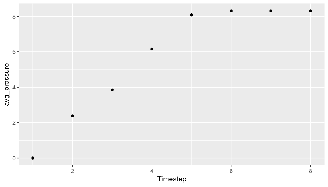

plot of chunk p-t-first-plot

Plot results for multiple simulations

# Get average pressure for all simulations
avg_pr_df <- storage_tbl %>%
  group_by(sim_id, timestep) %>%
  summarise(avg_pressure = mean(pressure))

# Plot pressure over time for all simulations
ggplot(avg_pr_df,
       aes(x = as.numeric(as.factor(timestep)),
           y = avg_pressure)) +
  geom_point(aes(color = as.factor(sim_id))) +
  geom_line(aes(color = as.factor(sim_id))) + 
  xlab("Timestep") + 
  labs(color = "sim id") +
  facet_grid(rows = vars(sim_id))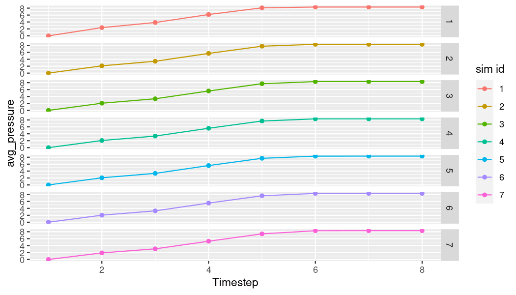

plot of chunk p-t-all-plot

Now we have the average pressure over time for each of the simulations (rows). Since they’re pretty similar, let’s put them in the same plot for a better comparison.

ggplot(avg_pr_df, aes(x = as.numeric(as.factor(timestep)),
                      y = avg_pressure,
                      group = sim_id)) +
  geom_point(aes(color = as.factor(sim_id))) +
  geom_line(aes(color = as.factor(sim_id))) + 
  labs(color = "sim id") +
  xlab("Timestep")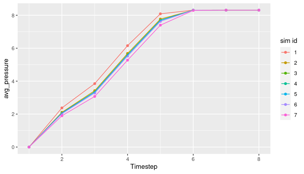

plot of chunk p-t-all-combined-plot

Multi-parameter sequential run

So far we’ve only considered the storage parameter. Now we want to have a look at how the other two parameters influence the simulation, so let’s put them into an ensemble together. For permeability we can reuse the percentages we already have. For porosity, this doesn’t work - the original value is 1 and its values can only range between 0 and 1, so we’ll supply a shorter vector.

This time it’s important we set the OGS6_Ensemble parameter sequential_mode to TRUE as this will change the supplied parameters sequentially which means in the end we have 18 (7 + 7 + 4) simulations which is equal to the sum of elements in the value vectors you supply (I’ve named them values below for clarity, naming them is optional though).

The default FALSE would give an error message because our value vectors do not have the same length and even if they had, it wouldn’t do what we want - the number of simulations would equal the length of one value vector (thus requiring them to be of the same length). Generally, set sequential_mode to TRUE if you want to examine the influence of parameters on a simulation independently. If you want to examine how the parameters influence each other as in wanting to test parameter combinations, the default mode is the way to go.

# Change this to fit your system
sim_path <- paste0(testdir_path, "/axisym_theis_sim_big")

ogs6_obj$sim_path <- sim_path

ogs6_ens_big <-
  OGS6_Ensemble$new(
    ogs6_obj = ogs6_obj,
    parameters = list(per = list(ogs6_obj$media[[1]]$properties[[1]]$value, 
                                 values = percentages),
                      por = list(ogs6_obj$media[[1]]$properties[[3]]$value, 
                                 c(-50, -10, -1, 0)),
                      sto = list(ogs6_obj$media[[1]]$properties[[4]]$value, 
                                 values = percentages)),
    sequential_mode = TRUE)

Now you can start the simulation.

ogs6_ens_big$run_simulation()

lapply(ogs6_ens_big$ensemble, ogs6_read_output_files)

This will take a short time. As soon as the simulations are done, we can extract the point data much like we did before. This time we want to plot the point x coodinates on the x axis so we’re leaving out point_ids to get all points. Also we just want the data from the last timestep.

# Get combined dataframe
per_por_sto_df <- 
  ogs6_ens_big$get_point_data(
    keys = c("pressure"),
    start_at_timestep = ogs6_ens_big$ensemble[[1]]$pvds[[1]]$last_timestep)

Plotting time! Since we set sequential_mode to TRUE, the dataframe we just created contains a name column which allows us to group by parameters. Because we’ve also set percentages_mode to TRUE, it also has a column perc which allows us to group by percentages. Now we can simply use a facet grid to plot.

# Make plot
ggplot(per_por_sto_df,
       aes(x = x,
           y = -pressure, # Flip pressure because source term was positive
           group = perc)) +
  geom_point(aes(color = as.factor(perc))) +
  xlab("Radius (m)") +
  ylab("Head (m)") +
  labs(color = "%") +
  facet_grid(cols = vars(name),
             labeller = as_labeller(c(per = "permeability",
                                      por = "porosity",
                                      sto =  "storage")))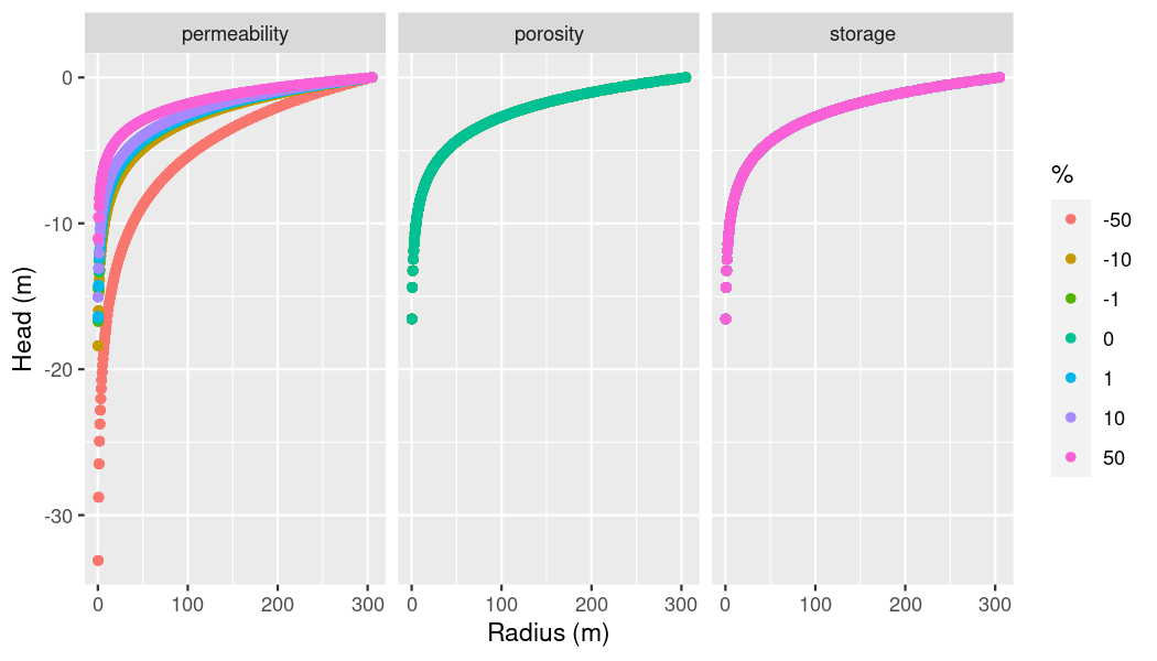

plot of chunk p-t-group-plot

Ta-Daa! We can see permeability has the most influence on the pressure. Though they may seem suspicious, porosity and storage are being plotted correctly - the points are just being placed right on top of each other. Since porosity can’t go over the value 1 which was the original value, our value vector only went from -50% to 0% which is why the line colors of porosity and storage differ. Maybe we want to try and use a logarithmic approach for storage. This won’t work with the built-in functionality of OGS6_Ensemble so we’ll set up our Ensemble a little differently.

# Calculate log value
log_val <- log(as.numeric(
  ogs6_obj$media[[1]]$properties[[4]]$value),
  base = 10)

# Apply changes to log value
log_vals <- vapply(percentages, function(x){
    log_val + (log_val * (x / 100))
}, FUN.VALUE = numeric(1))

# Transfer back to non-logarithmic scale
back_transf_vals <- 10^log_vals

# Change sim_path to fit your system
ogs6_obj$sim_path <- paste0(testdir_path, "/axisym_theis_sim_log_storage")

# Set up new ensemble
ogs6_ens_sto <-
    OGS6_Ensemble$new(
        ogs6_obj = ogs6_obj,
        parameters =
            list(
                sto = list(
                    ogs6_obj$media[[1]]$properties[[4]]$value,
                    values = back_transf_vals)
            ),
        percentages_mode = FALSE,
        sequential_mode = TRUE
    )

As before, we can run the simulation right away.

ogs6_ens_sto$run_simulation()

lapply(ogs6_ens_sto$ensemble, ogs6_read_output_files)

Let’s check if we can observe any influence of storage on pressure now.

# Get combined dataframe
sto_df <- 
    ogs6_ens_sto$get_point_data(
        keys = c("pressure"),
        start_at_timestep = ogs6_ens_sto$ensemble[[1]]$pvds[[1]]$last_timestep)

# Supply percentages manually since we couldn't use `percentages_mode`
percs <- vapply(sto_df$sim_id,
                function(x){percentages[[x]]},
                FUN.VALUE = numeric(1))

ggplot(sto_df,
       aes(x = x,
           y = -pressure)) +
    geom_point(aes(color = as.factor(percs))) +
    xlab("Radius (m)") +
    ylab("Head (m)") +
    labs(color = "%")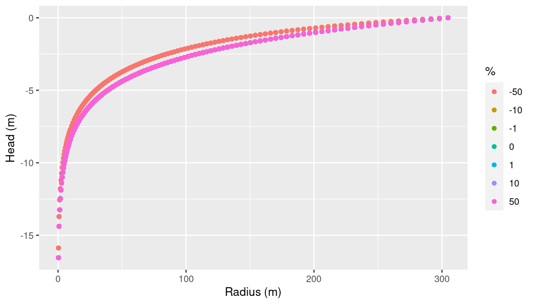

plot of chunk p-t-log-plot

Theis solution for well pumping

We will consider the following parameters for our sensitivity analysis:

permeability
porosity
slope

Setup

First, we create a simulation object to base our ensemble on and read in the .prj file. This time we want to specify that an output file only gets written at the last timestep.

# Change this to fit your system
sim_path <- paste0(testdir_path, "/theis_sim")

ogs6_obj <- OGS6$new(sim_name = "theis",
                     sim_path = sim_path)

# Change this to fit your system
prj_path <- system.file("extdata/benchmarks/theis_well_pumping/",
                        "theis.prj", package = "r2ogs6")

read_in_prj(ogs6_obj, prj_path, read_in_gml = T)

# Increase each_steps
ogs6_obj$time_loop$output$timesteps$pair$each_steps <- 200

Multi-parameter sequential run

# Assign percentages
percentages <- c(-50, -10, -1, 0, 1, 10, 50)

ogs6_ens_theis_2 <-
  OGS6_Ensemble$new(
    ogs6_obj = ogs6_obj,
    parameters =
      list(
        per = list(ogs6_obj$parameters[[3]]$values,
                   values = percentages),
        por = list(ogs6_obj$parameters[[2]]$value,
                   values = percentages),
        slo = list(
          ogs6_obj$media[[1]]$phases[[1]]$properties[[1]]$independent_variable[[2]]$slope,
          values = percentages)
      ),
    sequential_mode = TRUE
  )

Now you can start the simulation.

ogs6_ens_theis_2$run_simulation()

lapply(ogs6_ens_theis_2$ensemble, ogs6_read_output_files)

When the simulations have run, we can extract and plot the results like before. To avoid cluttering the plot, we only extract the pressure values for a single line. For this, we get the IDs of all points on the x axis.

# Extract point ids
get_point_ids_x <- function(points){
  x_axis_ids <- numeric()
  
  for(i in seq_len(dim(points)[[1]])) {
    if (points[i, ][[2]] == 0 && points[i, ][[3]] == 0) {
      x_axis_ids <- c(x_axis_ids, (i - 1))
    }
  }
  
  return(x_axis_ids)
}

point_ids_x <- get_point_ids_x(
  ogs6_ens_theis_2$ensemble[[1]]$pvds[[1]]$OGS6_vtus[[1]]$points)

# Get combined dataframe
per_por_slo_df <- 
  ogs6_ens_theis_2$get_point_data(
    point_ids = point_ids_x,
    keys = c("pressure"),
    start_at_timestep = ogs6_ens_theis_2$ensemble[[1]]$pvds[[1]]$last_timestep)

# Make plot
ggplot(per_por_slo_df,
       aes(x = x,
           y = pressure / 9806.65, # 1mH2O = 9806.65 kPa
           group = perc)) +
  geom_point(aes(color = as.factor(perc))) +
  xlab("Radius (m)") +
  ylab("Absenkung (m)") +
  labs(color = "%") +
  facet_grid(cols = vars(name),
             labeller = as_labeller(c(per = "permeability",
                                      por = "porosity",
                                      slo =  "slope"
                                      )))

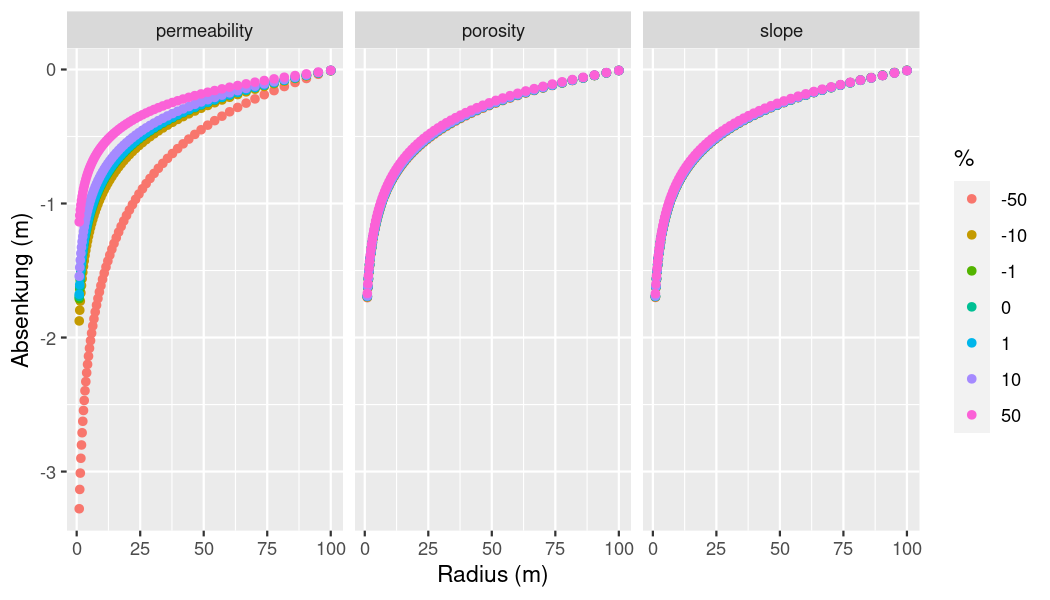
plot of chunk p-x-plot

Let’s take a closer look at permeability.

per_df <- subset(per_por_slo_df, name == "per")

# Make plot
ggplot(per_df,
       aes(x = x,
           y = pressure)) +
  geom_point(aes(color = as.factor(perc))) +
  xlab("Radius (m)") +
  ylab("Head (m)") +
  labs(color = "%")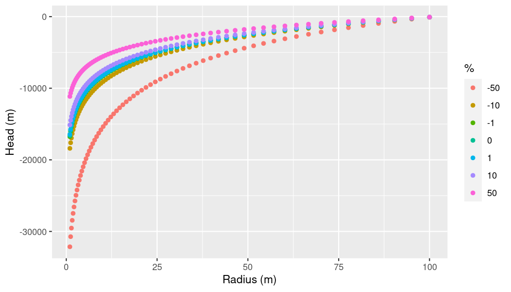

plot of chunk p-x-subset-plot

Maybe we want to try and use a logarithmic approach for slope. This won’t work with the built-in functionality of OGS6_Ensemble so we’ll set up our Ensemble a little differently.

# Calculate log value
log_val <- log(as.numeric(
  ogs6_obj$media[[1]]$phases[[1]]$properties[[1]]$independent_variable[[2]]$slope),
  base = 10)

# Apply changes to log value
log_vals <- vapply(percentages, function(x){
    log_val + (log_val * (x / 100))
}, FUN.VALUE = numeric(1))

# Transfer back to non-logarithmic scale
back_transf_vals <- 10^log_vals

# Change sim_path to fit your system
ogs6_obj$sim_path <- paste0(testdir_path, "/theis_sim_log_slope")

# Set up new ensemble
ogs6_ens_slo <-
    OGS6_Ensemble$new(
        ogs6_obj = ogs6_obj,
        parameters =
            list(
                slo = list(
                    ogs6_obj$media[[1]]$phases[[1]]$properties[[1]]$independent_variable[[2]]$slope,
                    values = back_transf_vals)
            ),
        percentages_mode = FALSE,
        sequential_mode = TRUE
    )

As before, we can run the simulation right away.

ogs6_ens_slo$run_simulation()

lapply(ogs6_ens_slo$ensemble, ogs6_read_output_files)

Let’s check if we can observe any influence of slope on pressure now.

# Filter point ids
point_ids_x <- get_point_ids_x(
  ogs6_ens_slo$ensemble[[1]]$pvds[[1]]$OGS6_vtus[[1]]$points)

# Get combined dataframe
slo_df <- 
    ogs6_ens_slo$get_point_data(
        point_ids = point_ids_x,
        keys = c("pressure"),
        start_at_timestep = ogs6_ens_slo$ensemble[[1]]$pvds[[1]]$last_timestep)

# Supply percentages manually since we couldn't use `percentages_mode`
percs <- vapply(slo_df$sim_id,
                function(x){percentages[[x]]},
                FUN.VALUE = numeric(1))

ggplot(slo_df,
       aes(x = x,
           y = pressure / 9806.65)) + # 1mH2O = 9806.65 kPa
    geom_point(aes(color = as.factor(percs))) +
    xlab("Radius (m)") +
    ylab("Head (m)") +
    labs(color = "%")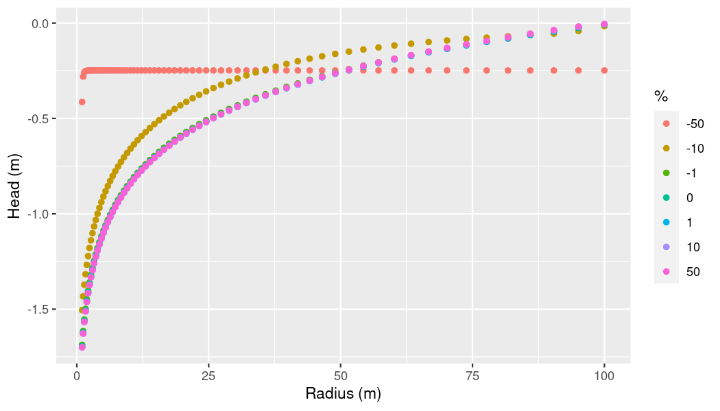

plot of chunk p-x-log-plot

Summary

The OGS6_Ensemble class is a useful tool to set up ensemble runs for sensitivity analyses. In this vignette, we learned how to create OGS6_Ensemble objects. We looked at how the parameters sequential_mode and percentages_mode influence how our ensemble object is initialised. We started simulations via OGS6_Ensemble$run_simulation() and extracted information from the output files to plot them.

2023-04-05

Introduction

Theis’ problem

Setup

Single-parameter sequential run

Plot results for single simulation

Plot results for multiple simulations

Multi-parameter sequential run

Theis solution for well pumping

Setup

Multi-parameter sequential run

Summary