User Guide
2023-04-05
user_workflow_vignette.RmdPrerequisites
This guide assumes you have r2ogs6 and its dependencies installed. If that’s not the case, please take a look at the installation instructions provided in the README.md file of the repository.
After loading r2ogs6, we first need to set the package options so it knows where to look for OpenGeoSys 6.
# Set path for OpenGeoSys 6
options("r2ogs6.default_ogs6_bin_path" = "your_ogs6_bin_path")
Creating your simulation object
To represent a simulation object, r2ogs6 uses an R6 class called OGS6. If you’re new to R6 objects, don’t worry. Creating a simulation object is easy. We call the class constructor and provide it with some parameters:
sim_nameThe name of your simulationsim_pathAll relevant files for your simulation will be in here
# Change this to fit your system
# sim_path <- system.file("extdata/benchmarks/flow_no_strain",
#                         package = "r2ogs6")
sim_path <- tempdir()
ogs6_obj <- OGS6$new(sim_name = "my_simulation",
                     sim_path = sim_path)
And that’s it, we now have a simulation object.
Defining the simulation parameters
From here on there’s two ways you can define the simulation parameters. Either you load a benchmark file or you define your simulation manually.
Loading a benchmark file
The quickest and easiest way to define a simulation is by using an already existing benchmark. If you take a look at the OpenGeoSys documentation, you’ll find plenty of benchmarks to choose from along with a link to their project file on GitLab at the top of the respective page.
For demonstration purposes, I will use a project from the HydroMechanics benchmarks, which can be found here.
# Change this to fit your system
#prj_path <- paste0(sim_path, "/flow_no_strain.prj")
prj_path <- system.file("extdata/benchmarks/flow_no_strain/flow_no_strain.prj",
                       package = "r2ogs6")
read_in_prj(ogs6_obj, prj_path = prj_path, read_in_gml = T)
NOTE: r2ogs6 has not been tested with every existing benchmark. Due to the large number of input parameters, you might encounter cases where the import fails.
Setting up your own OpenGeoSys 6 simulation
Setting up your own simulation is possible too.
Since there’s plenty of required and optional input parameters, you might want to call get_status() occasionally to get a brief overview of your simulation. This tells you which input parameters are missing before you can run a simulation.
# Call on the OGS6 object (note the R6 style)
ogs6_obj$get_status()
#> ✓ 'processes' has at least one element
#> ✓ 'time_loop' is defined
#> ✓ 'nonlinear_solvers' has at least one element
#> ✓ 'linear_solvers' has at least one element
#> ✓ 'parameters' has at least one element
#> ✓ 'process_variables' has at least one element
#> ✗ 'mesh' is defined
#> ✗ 'geometry' is defined
#> ✓ 'media' has at least one element
#> ✗ 'test_definition' has at least one element
#> ✗ 'curves' has at least one element
#> ✓ 'meshes' has at least one element
#> ✗ 'local_coordinate_system' is defined
#> ✗ 'search_length_algorithm' is defined
#> ✗ 'chemical_system' is defined
#> ✗ 'python_script' is defined
#> ✗ 'insitu' is definedYour OGS6 object has all necessary components.
#> You can try calling ogs6_run_simulation().Note that this calls more validation functions, so you may not be done just yet.
Since we haven’t defined anything so far, you’ll see a lot of red there. But the results gave us a hint what we can add. We’ll go from there and try to find out more about the possible input data. Say we want to find out more about process objects.
# To take a look at the documentation, use ? followed by the name of a class
?prj_process
As a rule of thumb, classes are named with the prefix prj_ followed by their XML tag name in the .prj file. The only exceptions to this rule are subclasses where this would lead to duplicate class names. The class prj_time_loop for example contains a subclass representing a process child element which is not to be confused with the process children of the first level processes node directly under the root node of the .prj file. Because of this, that subclass is named prj_tl_process. Let’s try adding something now.
To add data to our simulation object, we use OGS6$add(). We can use this method with any top level .prj element, which means we’re not limited to prj_parameter objects.
# Add a parameter
ogs6_obj$add(prj_parameter(name = "E",
                           type = "Constant",
                           value = 1e+10))


# Add a process variable
ogs6_obj$add(
    prj_process_variable(
        name = "pressure",
        components = 1,
        order = 1,
        initial_condition = "pressure0",
        boundary_conditions = list(
            boundary_condition = prj_boundary_condition(
                type = "Neumann",
                parameter = "flux_in",
                geometrical_set = "cube_1x1x1_geometry",
                geometry = "left",
                component = 0
            )
        )
    )
)
Since I already read in a .prj file earlier, I won’t run the above snippet. If you’d like a complete example of manually defining simulation parameters, there’s a script flow_free_expansion.R in the examples/workflow_demos folder.
Running the simulation
As soon as we’ve added all necessary parameters, we can try starting our simulation. This will run a few additional checks and then start OpenGeoSys 6. If write_logfile is set to FALSE, the output from OpenGeoSys 6 will be shown on the console.
ogs6_run_simulation(ogs6_obj)Retrieve the results
After our simulation is finished, we might want to plot some results. But how do we retrieve them? If all went as expected, we don’t need to call an extra function for that because ogs6_run_simulation() already calls ogs6_read_output_files() internally. We only need to decide what information we want to extract. Say we’re interested in the pressure Parameter from the last timestep. For this easy example, only one .pvd file was produced.
ogs6_read_output_files(ogs6_obj)
# Extract relevant info into dataframe
result_df <- ogs6_obj$pvds[[1]]$get_point_data(keys = c("pressure"))
result_df <- result_df[(result_df$timestep!=0),]

# Plot results
ggplot(result_df,
       aes(x = x,
           y = y,
           color = pressure)) +
    geom_point() +
    #geom_raster(interpolate = T)+
    #geom_contour_filled()+
    xlab("x coordinate") +
    ylab("y coordinate") +
    theme_bw()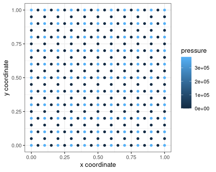
plot of chunk user-guide-plot
Similar to the idea with .pvd output, hdf5 files are automatically referenced under $h5s if returned by the simulation. Here, we have added a file artificially from the benchmark library for demonstration.
ogs6_obj$h5s
#> [[1]]
#> OGS6_h5
#> h5 path:
#> /work/ufz/r2ogs6/inst/extdata/benchmarks/EllipticPETSc/cube_1e3_np3.h5
#>
#> # h5 file structure ------------------------------------------------------
#>    group                   name       otype  dclass      dim
#> 0      /                    t_0   H5I_GROUP
#> 1   /t_0 D1_left_front_N1_right H5I_DATASET   FLOAT     1895
#> 2   /t_0     Linear_1_to_minus1 H5I_DATASET   FLOAT     1895
#> 3   /t_0            MaterialIDs H5I_DATASET INTEGER     1233
#> 4   /t_0               geometry H5I_DATASET   FLOAT 3 x 1895
#> 5   /t_0               pressure H5I_DATASET   FLOAT     1895
#> 6   /t_0               topology H5I_DATASET INTEGER    11097
#> 7   /t_0                      v H5I_DATASET   FLOAT 3 x 1895
#> 8      /                    t_1   H5I_GROUP
#> 9   /t_1               pressure H5I_DATASET   FLOAT     1895
#> 10  /t_1                      v H5I_DATASET   FLOAT 3 x 1895
As can be seen, hdf5 files have a very particular structure. To work with the data, a simple method get_h5() allows to access the different data elements as a very raw starting point for post processing the data.
h5_list <- ogs6_obj$h5s[[1]]$get_h5("/")Other functions such as HDF5 handles for dataset processing can be used directly from the rhdf5 package, of course. The path to the hd5 file is available as an active field h5_path that can be accessed or changed in the OGS6 object.
example_h5 <- rhdf5::H5Fopen(ogs6_obj$h5s[[1]]$h5_path)
example_h5
#> HDF5 FILE
#>         name /
#>     filename
#>
#>   name     otype dclass dim
#> 0  t_0 H5I_GROUP
#> 1  t_1 H5I_GROUP
str(example_h5$t_0)
#> List of 7
#>  $ D1_left_front_N1_right: num [1:1895(1d)] 1 1 1 1 1.01 ...
#>  $ Linear_1_to_minus1    : num [1:1895(1d)] 1 0.8 0.6 1 0.8 0.6 1 0.8 0.6 1 ...
#>  $ MaterialIDs           : int [1:1233(1d)] 0 0 0 0 0 0 0 0 0 0 ...
#>  $ geometry              : num [1:3, 1:1895] 0 0 0 0.1 0 0 0.2 0 0 0 ...
#>  $ pressure              : num [1:1895(1d)] 0 0 0 0 0 0 0 0 0 0 ...
#>  $ topology              : int [1:11097(1d)] 9 0 1 4 3 49 50 53 52 9 ...
#>  $ v                     : num [1:3, 1:1895] 0 0 0 0 0 0 0 0 0 0 ...
rhdf5::h5closeAll()
If the file has a reasonably “clean” structure, a more convenient way of importing the data is using the method get_df that returns a tibble table.
df <- ogs6_obj$h5s[[1]]$get_df(group = "/t_0", names = "pressure")
df
#> # A tibble: 1,895 × 5
#>        x     y     z  time pressure
#>    <dbl> <dbl> <dbl> <dbl>    <dbl>
#>  1   0     0       0     0        0
#>  2   0.1   0       0     0        0
#>  3   0.2   0       0     0        0
#>  4   0     0.1     0     0        0
#>  5   0.1   0.1     0     0        0
#>  6   0.2   0.1     0     0        0
#>  7   0     0.2     0     0        0
#>  8   0.1   0.2     0     0        0
#>  9   0.2   0.2     0     0        0
#> 10   0     0.3     0     0        0
#> # … with 1,885 more rows
Example Bechnmark with HDF5 output
Now this shows how to run a real example benchmark that outputs a hdf5 file. Setup and run the benchmark.
sim_path <- tempdir()
ogs6_obj2 <- OGS6$new("ex_hdf5", sim_path = sim_path)
prj_path <- system.file("extdata/benchmarks/square_1x1_SteadyStateDiffusion/square_1e2_GMRES_GML_output_xdmf-hdf5.prj",
                       package = "r2ogs6")
read_in_prj(ogs6_obj2, prj_path)

dir_make_overwrite(ogs6_obj2$sim_path)
run_benchmark(prj_path = prj_path, sim_path = ogs6_obj2$sim_path)
Now read the h5df output.
ogs6_read_output_files(ogs6_obj2)
h5_list <- ogs6_obj2$h5s[[1]]$get_h5("/")

h5_list
#> ogs6_obj2$h5s
# [[1]]
# OGS6_h5
# h5 path:
# /tmp/Rtmp4SkpPb/square_1x1_quad_1e2_GMRES_GML_output.h5

# h5 file structure ----------------------------------------------------------------------------------------------
                              group                     name       otype
#0                                 /                   meshes   H5I_GROUP
#1                           /meshes square_1x1_geometry_left   H5I_GROUP
#2  /meshes/square_1x1_geometry_left                 geometry H5I_DATASET
#3  /meshes/square_1x1_geometry_left                 pressure H5I_DATASET
#4  /meshes/square_1x1_geometry_left                 topology H5I_DATASET
#5  /meshes/square_1x1_geometry_left                        v H5I_DATASET
#6                           /meshes      square_1x1_quad_1e2   H5I_GROUP
#7       /meshes/square_1x1_quad_1e2                 geometry H5I_DATASET
#8       /meshes/square_1x1_quad_1e2                 pressure H5I_DATASET
#9       /meshes/square_1x1_quad_1e2                 topology H5I_DATASET
#10      /meshes/square_1x1_quad_1e2                        v H5I_DATASET
#11                                /                    times H5I_DATASET
#    dclass         dim
#0
#1
#2    FLOAT  3 x 11 x 1
#3    FLOAT      11 x 2
#4  INTEGER      40 x 1
#5    FLOAT  2 x 11 x 2
#6
#7    FLOAT 3 x 121 x 1
#8    FLOAT     121 x 2
#9  INTEGER     500 x 1
#10   FLOAT 2 x 121 x 2
#11   FLOAT           2
Running multiple simulations
If we want to run not one but multiple simulations, we can use the simulation object we just created as a blueprint for an ensemble run. The workflow for this is described in detail here.
Benchmark script generation
Another feature of r2ogs6 is benchmark script generation. For this, there are two functions.
ogs6_generate_benchmark_script()creates an R script from a.prjfileogs6_generate_benchmark_scripts()is a wrapper for the former. Instead of a single.prjfile path, it takes a directory path as its argument.
Let’s look at the parameters for ogs6_generate_benchmark_script() first. Say we have a project file sim_file.prj we want to generate a script from. Please, make sure that all the directories your are referencing exist.
# The path to the project file you want to generate a script from
prj_path <- "your_path/sim_file.prj"

# The path you want to save the simulation files to
sim_path <- "your_sim_directory/"

# The path to your `ogs.exe` (if not already specified in `r2ogs6` options)
ogs6_bin_path <- "your_ogs6_bin_path/"

# The path you want your benchmark script to be saved to
script_path <- "your_script_directory/"
Now that we have defined our parameters, we can generate the benchmark script.
ogs6_generate_benchmark_script(prj_path = prj_path,
                               sim_path = sim_path,
                               ogs6_bin_path = ogs6_bin_path,
                               script_path = script_path)
On the other hand, if we want to generate R scripts from multiple (or all) benchmarks, we can use the wrapper function ogs6_generate_benchmark_scripts(). Its parameters are basically the same, only this time we supply it with a directory path instead of a .prj path to start from.
You can download the benchmarks (or the subfolder you need) from here and then set path to their location on your system.
# The path to the directory you want to generate R scripts from
path <- "path/to/ogs/Tests/Data/Elliptic/"

# The path you want to save the simulation files to
sim_path <- "your_sim_directory/"

# The path you want your benchmark scripts to be saved to
script_path <- sim_path

# Optional: Use if you want to start from a specific `.prj` file
starting_from_prj_path <- ""

# Optional: Use if you want to skip specific `.prj` files
skip_prj_paths <- character()

# Optional: Use if you want to skip specific `.prj` files
skip_prj_paths <- character()

# Optional: Use if you want to restrict scripting to specific `.prj` files
only_prj_files <- character()
And we’re set! Note that ogs6_generate_benchmark_scripts() will reconstruct the structure of the folder your benchmarks are stored in, e. g. if there’s a file path/a/file.prj, you will find the corresponding R script in sim_path/a/file.R.
ogs6_generate_benchmark_scripts(path = path,
                                sim_path = sim_path,
                                script_path = script_path,
                                starting_from_prj_path = starting_from_prj_path,
                                skip_prj_paths = skip_prj_paths,
                                only_prj_files = only_prj_files)
With this, we can generate scripts from all benchmarks in a single call. Of course you can modify path to your liking if you’re only interested in generating scripts from certain subfolders.
Furthermore, you can restrict the script generation to benchmarks that used as test in OGS 6.
# extract *.prj files that are used as tests
rel_testbm_paths <- get_benchmark_paths("path/to/ogs-source-code/ProcessLib/")
rel_testbm_paths <- sapply(rel_testbm_paths, basename)

ogs6_generate_benchmark_scripts(path = path,
                                sim_path = sim_path,
                                script_path = script_path,
                                only_prj_files = rel_testbm_paths)
NOTE: New benchmarks and .prj parameters are constantly being added to OGS6. If a benchmark contains parameters that have not been added to r2ogs6 yet, the script generation functions will not work. If this is the case, they will be skipped and the original error message will be displayed in the console.